library(tidyverse)
library(tidyquant)
library(patchwork)
library(scales)
library(writexl)
library(zoo)
library(moments)

library(rugarch); library(broom)

library(gt)Contents
- Volatility as annualized standard deviation
- Varies by frequency (periodicity) and window
- Exponentially weighted moving average (EWMA)
- GARCH(1,1)
- The actual returns are non-normal (heavy-tailed)
Load packages
Volatility as annualized standard deviation
Retrieve prices, calculate log returns and create all_returns_* dataframe
# symbols <- c("PG", "JPM", "NVDA")
# mult_stocks <- tq_get(symbols, get = "stock.prices", from = "2010-12-31", to = "2023-11-09")
# mult_stocks$symbol <- mult_stocks$symbol <- factor(mult_stocks$symbol, levels = c("PG", "JPM", "NVDA"))
# saveRDS(mult_stocks, "mult_stocks.rds")

mult_stocks <- readRDS("mult_stocks.rds")

# tq_mutate_fun_options() returns list of compatible mutate functions by pkg

calculate_returns <- function(data, period) {
  data |>
    group_by(symbol) |>
    tq_transmute(select = adjusted,
                 mutate_fun = periodReturn,
                 period = period,
                 type = "log")
}

periods <- c("daily", "weekly", "monthly", "quarterly", "yearly")

# all_returns_daily <- calculate_returns(mult_stocks, "daily")
# all_returns_weekly <- calculate_returns(mult_stocks, "weekly")
# all_returns_monthly <- calculate_returns(mult_stocks, "monthly")
# all_returns_quarterly <- calculate_returns(mult_stocks, "quarterly")

all_returns <- set_names(periods) |> map(~ calculate_returns(mult_stocks, .x))
all_returns <- map(all_returns, ~ .x %>%
                                     group_by(symbol) %>%
                                     arrange(date) %>%  # Sort by date within each group
                                     slice(-1) %>%      # Remove the first row for each group
                                     ungroup())

all_returns_daily     <- all_returns$daily
all_returns_weekly    <- all_returns$weekly
all_returns_quarterly <- all_returns$quarterly
all_returns_monthly   <- all_returns$monthly
Save to Excel (to manually check calcualtions). But after first time, eval = FALSE
write_xlsx(all_returns, path = "all_returns.xlsx")

# This assumes 'all_returns' is a named list of data frames
# and each data frame has a 'symbol' column for stock tickers

# Step 1: Split each data frame by 'symbol' and create a named list of data frames
all_returns_by_stock <- map(all_returns, function(df) {
  split(df, df$symbol)
})

# Step 2: Name each data frame according to the period and stock
all_returns_by_stock <- imap(all_returns_by_stock, function(df_list, period_name) {
  set_names(df_list, paste(period_name, names(df_list), sep = "_"))
})

# Flatten the list of lists into a single list of data frames
all_returns_by_stock_flat <- flatten(all_returns_by_stock)

# Step 3 and 4: Write the list of data frames to an Excel file
write_xlsx(all_returns_by_stock_flat, path = "all_returns_by_stock.xlsx")
Different frequencies but the same (four year) window
calc_rolling_sd <- function(data, return_col_name, window_width) {
  data |>
        group_by(symbol) |>
        mutate(rolling_sd = rollapply(get(return_col_name),
                                      width = window_width,
                                      FUN = sd,
                                      align = "right", fill = NA)) |>
        ungroup()
}

#  Window lengths for each frequency (aka, periodicity)
W.daily     <- 250 * 4
W.weekly    <- 52 * 4
W.monthly   <- 12 * 4
W.quarterly <- 4 * 4

all_returns_daily <- calc_rolling_sd(all_returns_daily, "daily.returns", W.daily)
all_returns_weekly <- calc_rolling_sd(all_returns_weekly, "weekly.returns", W.weekly)
all_returns_monthly <- calc_rolling_sd(all_returns_monthly, "monthly.returns", W.monthly)
all_returns_quarterly <- calc_rolling_sd(all_returns_quarterly, "quarterly.returns", W.quarterly)
Still different frequencies (aka, periodicity) but annualized
# Function to calculate annualized volatility and add frequency
calc_annualized_vol <- function(df, sd_col, periods_per_year, freq_label) {
  df |>
        mutate(
            annualized_vol = !!rlang::sym(sd_col) * sqrt(periods_per_year),
            frequency = freq_label
    )
}

# Calculate annualized volatility for each dataframe EXCEPT Quarterly
all_returns_daily <- calc_annualized_vol(all_returns_daily, "rolling_sd", 252, "Daily")
all_returns_weekly <- calc_annualized_vol(all_returns_weekly, "rolling_sd", 52, "Weekly")
all_returns_monthly <- calc_annualized_vol(all_returns_monthly, "rolling_sd", 12, "Monthly")

# Combine the data frames into one
all_returns_combined <- bind_rows(all_returns_daily, all_returns_weekly, all_returns_monthly)
all_returns_combined <- all_returns_combined |>
    mutate(frequency = factor(frequency, levels = c("Daily", "Weekly", "Monthly")))

# Plot the combined data with ggplot2

color_pg <- "chartreuse2" # don't end up using these
color_jpm <- "dodgerblue2"
color_nvda <- "coral1"

color_tenor1 <- "khaki3"
color_tenor2 <- "coral"
color_tenor3 <- "lightseagreen"
color_tenor4 <- "slateblue"

custom_colors <- c("Daily" = color_tenor1, "Weekly" = color_tenor2, "Monthly" = color_tenor3)

all_returns_combined |> ggplot(aes(x = date, y = annualized_vol,
                                   color = frequency,
                                   group = interaction(symbol, frequency))) +
    geom_line() +
    labs(title = "Annualized Volatility by Frequency",
         x = "Date",
         y = "Annualized Volatility") +
    theme_minimal() +
    scale_color_manual(values = custom_colors) +
    facet_wrap(~symbol)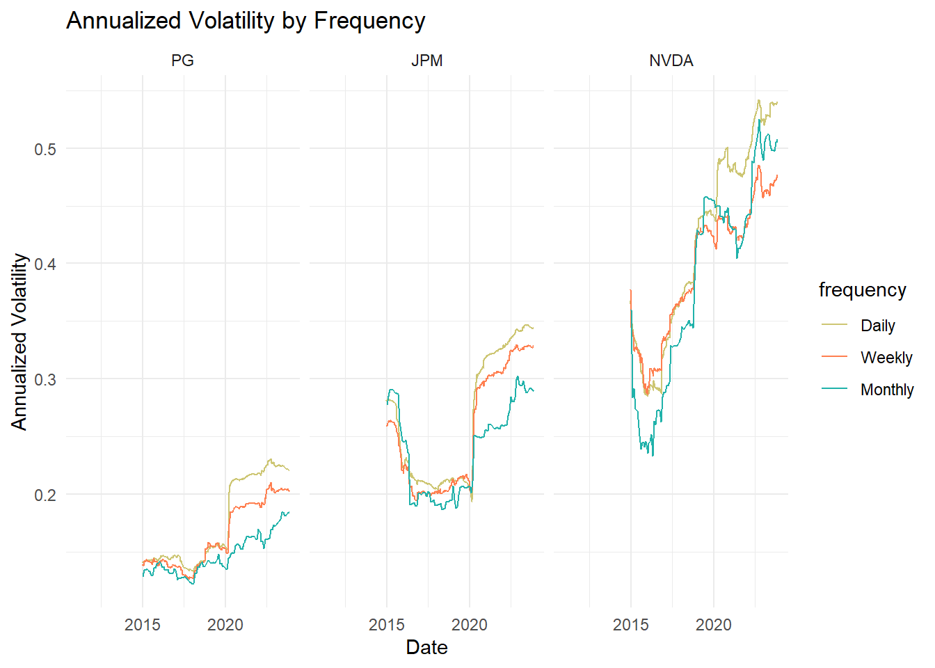
# mean annualized vol by symbol and frequency
all_returns_combined |>
    group_by(symbol, frequency) |>
    summarize(annualized_vol = mean(annualized_vol, na.rm = TRUE)) |>
    pivot_wider(names_from = frequency, values_from = annualized_vol) |>
    arrange(Daily)
# A tibble: 3 × 4
# Groups: symbol [3]
symbol Daily Weekly Monthly
<fct> <dbl> <dbl> <dbl>
1 PG 0.176 0.164 0.147
2 JPM 0.265 0.255 0.239
3 NVDA 0.421 0.396 0.388Different windows but same (DAILY) frequency
# colors from my var article
# col_ticker_fills <- c("PG" = "chartreuse2", "JPM" = "dodgerblue2", "NVDA" = "coral1")

windows <- c(20, 90, 250, 500)

# parse into per-ticker df and delete rolling_sd column from prior
pg_data   <- all_returns_daily |> filter(symbol == "PG")   |> select(!rolling_sd)
jpm_data  <- all_returns_daily |> filter(symbol == "JPM")  |> select(!rolling_sd)
nvda_data <- all_returns_daily |> filter(symbol == "NVDA") |> select(!rolling_sd)

# Specify your window sizes directly in the loop
for (w in windows) {
  pg_data <- pg_data |>
      mutate(!!paste0("rolling_sd_", w) := rollapply(daily.returns,
                                                     width = w,
                                                     FUN = sd,
                                                     align = "right", fill = NA))
  jpm_data <- jpm_data |>
      mutate(!!paste0("rolling_sd_", w) := rollapply(daily.returns,
                                                     width = w,
                                                     FUN = sd,
                                                     align = "right", fill = NA))
  nvda_data <- nvda_data |>
      mutate(!!paste0("rolling_sd_", w) := rollapply(daily.returns,
                                                     width = w,
                                                     FUN = sd,
                                                     align = "right", fill = NA))
}

plot_rolling_sd <- function(data, stock_name, ylim, custom_colors, custom_alphas) {
    # Assume data has columns 'date', and rolling_sd_* where * is the window size
    rolling_sd_long <- data |>
        pivot_longer(cols = starts_with("rolling_sd_"), names_to = "window", values_to = "rolling_sd")
    desired_order <- c("rolling_sd_20", "rolling_sd_90", "rolling_sd_250", "rolling_sd_500")
    rolling_sd_long$window <- factor(rolling_sd_long$window, levels = desired_order)
    ggplot(rolling_sd_long, aes(x = date, y = rolling_sd, color = window)) +
        geom_line(aes(alpha = window)) +
        scale_color_manual(values = custom_colors) +
        scale_alpha_manual(values = custom_alphas) +
        labs(title = paste("Rolling Daily Vol (StdDev) for", stock_name),
             subtitle = paste("Different windows:", paste(windows, collapse = ", "), "days"),
             x = "Date",
             y = "Rolling Standard Deviation") +
        theme_minimal() +
        coord_cartesian(ylim = ylim) +
        theme(legend.position = "right")
}

# custom_colors <- c("rolling_sd_20" = "firebrick1",
#                   "rolling_sd_90" = "royalblue",
#                   "rolling_sd_250" = "springgreen4",
#                   "rolling_sd_500" = "darkorange")

custom_colors <- c("rolling_sd_20" = color_tenor1,
                   "rolling_sd_90" = color_tenor2,
                   "rolling_sd_250" = color_tenor3,
                   "rolling_sd_500" = color_tenor4)

custom_alphas <- c("rolling_sd_20" = 0.5,
                   "rolling_sd_90" = 0.7,
                   "rolling_sd_250" = 1.0,
                   "rolling_sd_500" = 1.0)

pg_roll_plot <- plot_rolling_sd(pg_data, "PG", c(0, 0.0350), custom_colors, custom_alphas)
jpm_roll_plot <- plot_rolling_sd(jpm_data, "JPM", c(0, 0.0550), custom_colors, custom_alphas)
nvda_roll_plot <- plot_rolling_sd(nvda_data, "NVDA", c(0, 0.0750), custom_colors, custom_alphas)

pg_roll_plot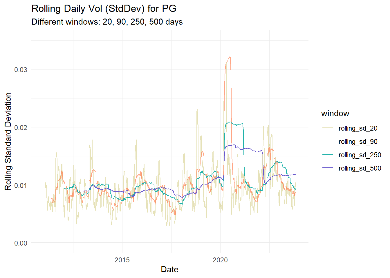
jpm_roll_plot
nvda_roll_plot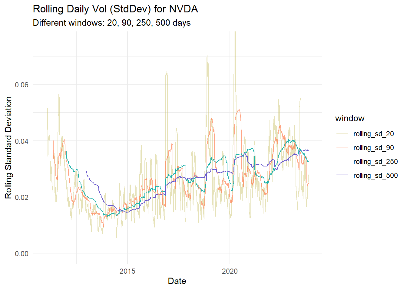
# Function to summarize and extract the most recent rolling standard deviations

summarize_and_extract_recent_sd <- function(data) {
  summarized <- data %>%
    summarize(
      mean_sd_20 = mean(rolling_sd_20, na.rm = TRUE),
      mean_sd_90 = mean(rolling_sd_90, na.rm = TRUE),
      mean_sd_250 = mean(rolling_sd_250, na.rm = TRUE),
      mean_sd_500 = mean(rolling_sd_500, na.rm = TRUE)
    )

  most_recent <- data %>%
    slice(n()) %>%
    select(rolling_sd_20, rolling_sd_90, rolling_sd_250, rolling_sd_500) %>%
    rename(recent_sd_20 = rolling_sd_20,
           recent_sd_90 = rolling_sd_90,
           recent_sd_250 = rolling_sd_250,
           recent_sd_500 = rolling_sd_500)

  bind_cols(summarized, most_recent)
}

# Apply the function to each data frame and bind rows into a single tibble
summary_tibble <- bind_rows(
  pg = summarize_and_extract_recent_sd(pg_data),
  jpm = summarize_and_extract_recent_sd(jpm_data),
  nvda = summarize_and_extract_recent_sd(nvda_data),
  .id = "stock"
)

summary_tibble |>
    gt() |>
    tab_header(
        title = "Rolling daily volatility"
    ) |>
    cols_label(
        mean_sd_20 = "20",
        mean_sd_90 = "90",
        mean_sd_250 = "250",
        mean_sd_500 = "500",
        recent_sd_20 = "20",
        recent_sd_90 = "90",
        recent_sd_250 = "250",
        recent_sd_500 = "500"
    ) |>
    fmt_percent(columns = 2:9,
                rows = everything()) |>
    tab_spanner(
        label = "Mean",
        columns = 2:5
    ) |>
    tab_spanner(
        label = "Most recent (2023-11-08)",
        columns = 6:9
    ) |>
    cols_width(
        mean_sd_20 ~ px(80),
        recent_sd_20 ~ px(80)
    ) |>
    data_color(
        columns = 6:9,
        rows = 3,
        method = "numeric",
        domain = c(0.02, 0.04),
        palette = c("lightcyan", "lightcyan3")
)| Rolling daily volatility | ||||||||
|---|---|---|---|---|---|---|---|---|
| stock | Mean | Most recent (2023-11-08) | ||||||
| 20 | 90 | 250 | 500 | 20 | 90 | 250 | 500 | |
| pg | 0.98% | 1.03% | 1.07% | 1.09% | 0.96% | 0.86% | 0.93% | 1.18% |
| jpm | 1.53% | 1.61% | 1.66% | 1.66% | 1.26% | 1.01% | 1.36% | 1.64% |
| nvda | 2.54% | 2.64% | 2.66% | 2.64% | 2.76% | 2.47% | 3.25% | 3.63% |
# GPT wrote this routine to summarize!

summarize_rolling_sd <- function(data) {
  # Define the desired order for the window sizes
  window_order <- c("rolling_sd_20", "rolling_sd_90", "rolling_sd_250", "rolling_sd_500")

  summarized_data <- data %>%
    summarize(across(starts_with("rolling_sd_"), mean, na.rm = TRUE)) %>%
    pivot_longer(cols = everything(), names_to = "window", values_to = "rolling_sd") %>%
    mutate(window = factor(window, levels = window_order)) %>%
    arrange(window)

  return(summarized_data)
}

# Apply the summarize function to each stock and combine into a single tibble
all_summaries <- bind_rows(
  pg = summarize_rolling_sd(pg_data),
  jpm = summarize_rolling_sd(jpm_data),
  nvda = summarize_rolling_sd(nvda_data),
  .id = "stock"
)

# Print the combined summarized data
print(all_summaries)
# A tibble: 12 × 3
stock window rolling_sd
<chr> <fct> <dbl>
1 pg rolling_sd_20 0.00977
2 pg rolling_sd_90 0.0103
3 pg rolling_sd_250 0.0107
4 pg rolling_sd_500 0.0109
5 jpm rolling_sd_20 0.0153
6 jpm rolling_sd_90 0.0161
7 jpm rolling_sd_250 0.0166
8 jpm rolling_sd_500 0.0166
9 nvda rolling_sd_20 0.0254
10 nvda rolling_sd_90 0.0264
11 nvda rolling_sd_250 0.0266
12 nvda rolling_sd_500 0.0264 Exponentially weighted moving average (EWMA)
# Function to calculate EWMA variance
calculate_ewma_variance <- function(returns, lambda, W) {
    ewma_var <- rep(NA, length(returns))
    ewma_var[W] <- var(returns[1:W])  # Initialize the first EWMA variance
    for (i in (W+1):length(returns)) {
        # Using the EWMA formula
        ewma_var[i] <- lambda * ewma_var[i-1] + (1 - lambda) * returns[i]^2
    }
    return(ewma_var)
}

# Example lambda value
W       <- 250
lambda  <- 0.94

# Use rollapply with your custom EWMA function
# Assuming the 'returns' column in all_returns_daily is the daily return for each stock
all_returns_daily <- all_returns_daily |>
    group_by(symbol) |>
    mutate(ewma_variance = calculate_ewma_variance(daily.returns, lambda, W)) |>
    ungroup()

# Calculate the EWMA volatility from the EWMA variance
all_returns_daily <- all_returns_daily |>
    mutate(ewma_sd = sqrt(ewma_variance))

# Reshape the data to long format for ggplot2
all_returns_long <- all_returns_daily |>
    pivot_longer(cols = c("rolling_sd", "ewma_sd"),
                 names_to = "sd_type",
                 values_to = "sd_value")

# Plot the data with ggplot2
custom_sd_colors <- c("rolling_sd" = color_tenor4, "ewma_sd" = color_tenor2)

all_returns_long |> ggplot (aes(x = date, y = sd_value, color = sd_type)) +
    geom_line(aes(alpha = sd_type)) +
    scale_color_manual(values = custom_sd_colors) +
    scale_alpha_manual(values = c(0.5, 1.0)) +
    labs(title = "EWMA is much more reactive than unweighted StdDev",
         subtitle = "(rolling_sd window = 250 days * 4 years = 1000 days)",
         x = "Date",
         y = "Standard Deviation") +
    facet_wrap(~symbol) +
    coord_cartesian(ylim = c(0, 0.050)) +
    theme_minimal() +
    theme(legend.position = "bottom")
Let’s compare different lambda (aka, smoothing) parameters
library(dplyr)
library(ggplot2)
library(tidyr)

plot_ewma_for_stock <- function(data, symbol, returns_col, lambda_list,
                                custom_colors, custom_alphas, ylim) {

    # Function to calculate EWMA variance - make sure this is defined in your environment
    calculate_and_store_ewma <- function(data, symbol, returns_col, lambda_list) {

        for (lambda in lambda_list) {
            W = 250
            lambda <- lambda
            ewma_col_name <- paste0("lambda_", as.character(lambda))
            data <- data |>
                mutate(
                    !!ewma_col_name := sqrt(calculate_ewma_variance(get(returns_col), lambda, W))
                )
            }
        return(data)
        }

    # Calculate and store EWMA with multiple parameters for the specified stock
    stock_ewma <- calculate_and_store_ewma(data, symbol, returns_col, lambda_list)

    # Pivot the data to long format for plotting
    stock_ewma_long <- stock_ewma |>
        pivot_longer(cols = starts_with("lambda"), names_to = "lambda", values_to = "ewma_sd")

    # Plot the EWMA standard deviations for different parameter sets
    gg <- ggplot(stock_ewma_long, aes(x = date, y = ewma_sd, color = lambda)) +
        geom_line(aes(alpha = lambda)) +
        scale_color_manual(values = custom_colors) +
        scale_alpha_manual(values = custom_alphas) +
        labs(title = paste("EWMA volatility for", symbol, "with Different Parameters"),
             x = "Date",
             y = "EWMA Standard Deviation") +
        coord_cartesian(ylim = c(0, ylim)) +
        theme_minimal() +
        theme(legend.position = "right")

  return(gg)
}

# Define the sets of parameters you want to compare
lambda_list <- c(0.91, 0.94, 0.97)

# custom_colors <- c("lambda_0.91" = "firebrick1",
#                   "lambda_0.94" = "royalblue",
#                   "lambda_0.97" = "springgreen4")

custom_colors <- c("lambda_0.91" = color_tenor1,
                   "lambda_0.94" = color_tenor2,
                   "lambda_0.97" = color_tenor4)

custom_alphas <- c("lambda_0.91" = 0.6,
                   "lambda_0.94" = 0.8,
                   "lambda_0.97" = 1.0)

jpm_ewma_plot <- plot_ewma_for_stock(jpm_data, "JPM", "daily.returns", lambda_list,
                                custom_colors, custom_alphas, 0.080)
pg_ewma_plot <- plot_ewma_for_stock(pg_data, "PG", "daily.returns", lambda_list,
                               custom_colors, custom_alphas, 0.0550)
nvda_ewma_plot <- plot_ewma_for_stock(nvda_data, "NVDA", "daily.returns", lambda_list,
                                 custom_colors, custom_alphas, 0.070)

jpm_ewma_plot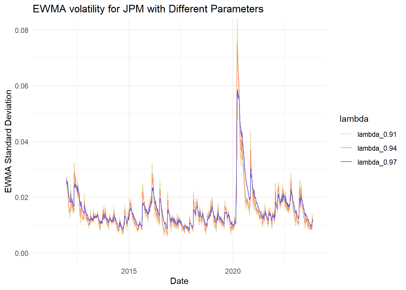
pg_ewma_plot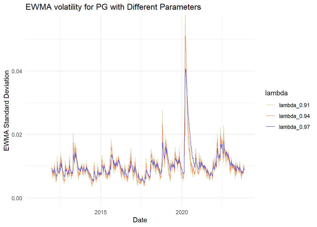
nvda_ewma_plot
GARCH(1,1)
Fitting the parameters
# library(rugarch)
# Define the GARCH(1,1) specification outside the loop to avoid redundancy
spec <- ugarchspec(variance.model = list(model = "sGARCH", garchOrder = c(1, 1)),
                   mean.model = list(armaOrder = c(0, 0), include.mean = TRUE),
                   distribution.model = "norm")

# Fit the GARCH(1,1) model for each stock symbol
garch_models <- all_returns_daily |>
    group_by(symbol) |>
    nest() |>
    mutate(model = map(data, ~ ugarchfit(spec, data = .$daily.returns)))

# Manual extraction of coefficients
garch_coef_manual <- garch_models |>
    mutate(coef = map(model, function(m) as.data.frame(t(coef(m))))) |>
    select(symbol, coef) |>
    unnest(coef)

garch_coef_manual <- garch_coef_manual |> ungroup()
garch_coef_manual <- garch_coef_manual |> mutate(
    gamma = 1 - alpha1 - beta1,
    LR_vol = sqrt(omega / (1 - alpha1 - beta1))
    )

garch_coef_manual |> select(-mu) |>
    gt(rowname_col = "symbol") |>
    fmt_scientific(columns = 2) |>
fmt_number(columns = 3:6, decimals = 4) | omega | alpha1 | beta1 | gamma | LR_vol | |
|---|---|---|---|---|---|
| PG | 1.06 × 10⁻⁵ | 0.1310 | 0.7744 | 0.0946 | 0.0106 |
| JPM | 9.31 × 10⁻⁶ | 0.0994 | 0.8659 | 0.0347 | 0.0164 |
| NVDA | 3.28 × 10⁻⁵ | 0.1006 | 0.8628 | 0.0366 | 0.0300 |
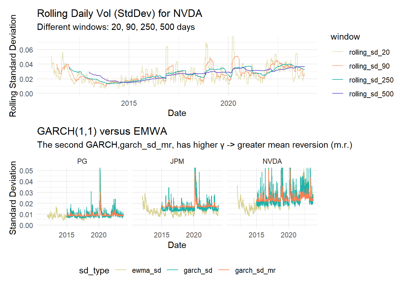
Plotting GARCH(1,1) volatility
# Function to calculate GARCH(1,1) variance
calculate_garch_variance <- function(returns, alpha, beta, gamma, W) {
    long_run_variance <- var(returns[1:W], na.rm = TRUE)
    omega <- gamma * long_run_variance
    garch_var <- rep(NA, length(returns))
    garch_var[W] <- var(returns[1:W])  # Initialize the first GARCH variance

    for (i in (W+1):length(returns)) {
        garch_var[i] <- omega + alpha * returns[i]^2 + beta * garch_var[i-1]
    }

    return(garch_var)
}

alpha <- 0.12; beta <- 0.78; gamma <- 1 - alpha - beta
alpha_mr <- 0.03; beta_mr <- 0.83; gamma_mr <- 1 - alpha_mr - beta_mr

# Calculate rolling GARCH(1,1) variance
all_returns_daily <- all_returns_daily |>
  group_by(symbol) |>
  mutate(garch_variance   = calculate_garch_variance(daily.returns, alpha, beta,
                                                   gamma, W.daily),
         garch_variance_mr = calculate_garch_variance(daily.returns, alpha_mr, beta_mr,
                                                     gamma_mr, W.daily))  |>
  ungroup()

# Calculate the GARCH(1,1) standard deviation from the GARCH variance
all_returns_daily <- all_returns_daily |>
    mutate(garch_sd = sqrt(garch_variance),
           garch_sd_mr = sqrt(garch_variance_mr))

all_returns_long <- all_returns_daily |>
    pivot_longer(cols = c("garch_sd", "garch_sd_mr", "ewma_sd"),
                 names_to = "sd_type", values_to = "sd_value")


custom_line_colors <- c("garch_sd" = color_tenor3,
                        "garch_sd_mr" = color_tenor2,
                        "ewma_sd" = color_tenor1)
custom_line_alphas <- c("garch_sd" = 1.0,
                        "garch_sd_mr" = 1.0,
                        "ewma_sd" = 0.8)

# Plot the data with ggplot2
garch_p1 <- ggplot(all_returns_long, aes(x = date, y = sd_value, color = sd_type)) +
  geom_line(aes(alpha = sd_type)) +
    scale_color_manual(values = custom_line_colors) +  # Set custom colors
    scale_alpha_manual(values = custom_line_alphas) +  # Set custom alphas
  labs(title = "GARCH(1,1) versus EMWA",
       subtitle = "The second GARCH,garch_sd_mr, has higher γ -> greater mean reversion (m.r.)",
       x = "Date",
       y = "Standard Deviation") +
    facet_wrap(~symbol) +
    coord_cartesian(ylim = c(0, 0.05)) +
  theme_minimal() +
  theme(legend.position = "bottom")

garch_p1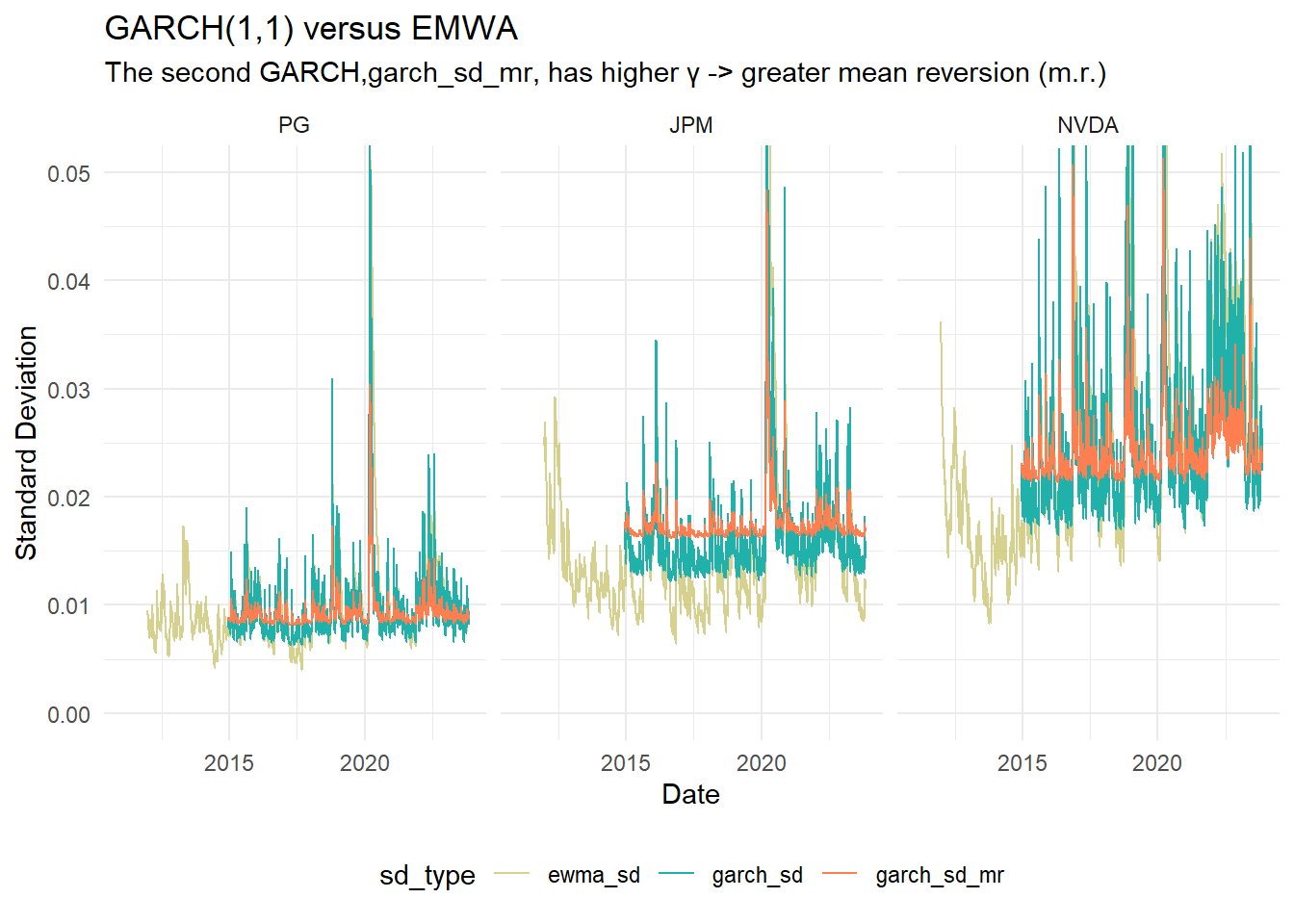
None of the returns are nearly normal
plot_histogram_with_normal <- function(stock_data, symbol, return_col) {
    # Calculate mean and standard deviation of returns
    mean_return <- mean(stock_data[[return_col]], na.rm = TRUE)
    sd_return <- sd(stock_data[[return_col]], na.rm = TRUE)

    binwidth <- (max(stock_data[[return_col]], na.rm = TRUE) -
                     min(stock_data[[return_col]], na.rm = TRUE)) / 120
    # print(binwidth) experimenting with binwidth

    # Create the histogram and overlay the normal distribution
    ggplot(stock_data, aes_string(x = return_col)) +
        geom_histogram(aes(y = ..density..), binwidth = binwidth,
                       color = "coral", fill = "khaki3", alpha = 0.6) +
        stat_function(fun = dnorm, args = list(mean = mean_return, sd = sd_return),
                      color = "slateblue", size = 1) +
        labs(title = paste("Histogram of Returns with Normal Distribution for", symbol),
             x = "Returns",
             y = "Density") +
        theme_minimal() +
        coord_cartesian(xlim = c(-0.1, 0.1))
}

jpm_hist_plot <- plot_histogram_with_normal(jpm_data, "JPM", "daily.returns")
pg_hist_plot <- plot_histogram_with_normal(pg_data, "PG", "daily.returns")
nvda_hist_plot <- plot_histogram_with_normal(nvda_data, "NVDA", "daily.returns")

jpm_hist_plot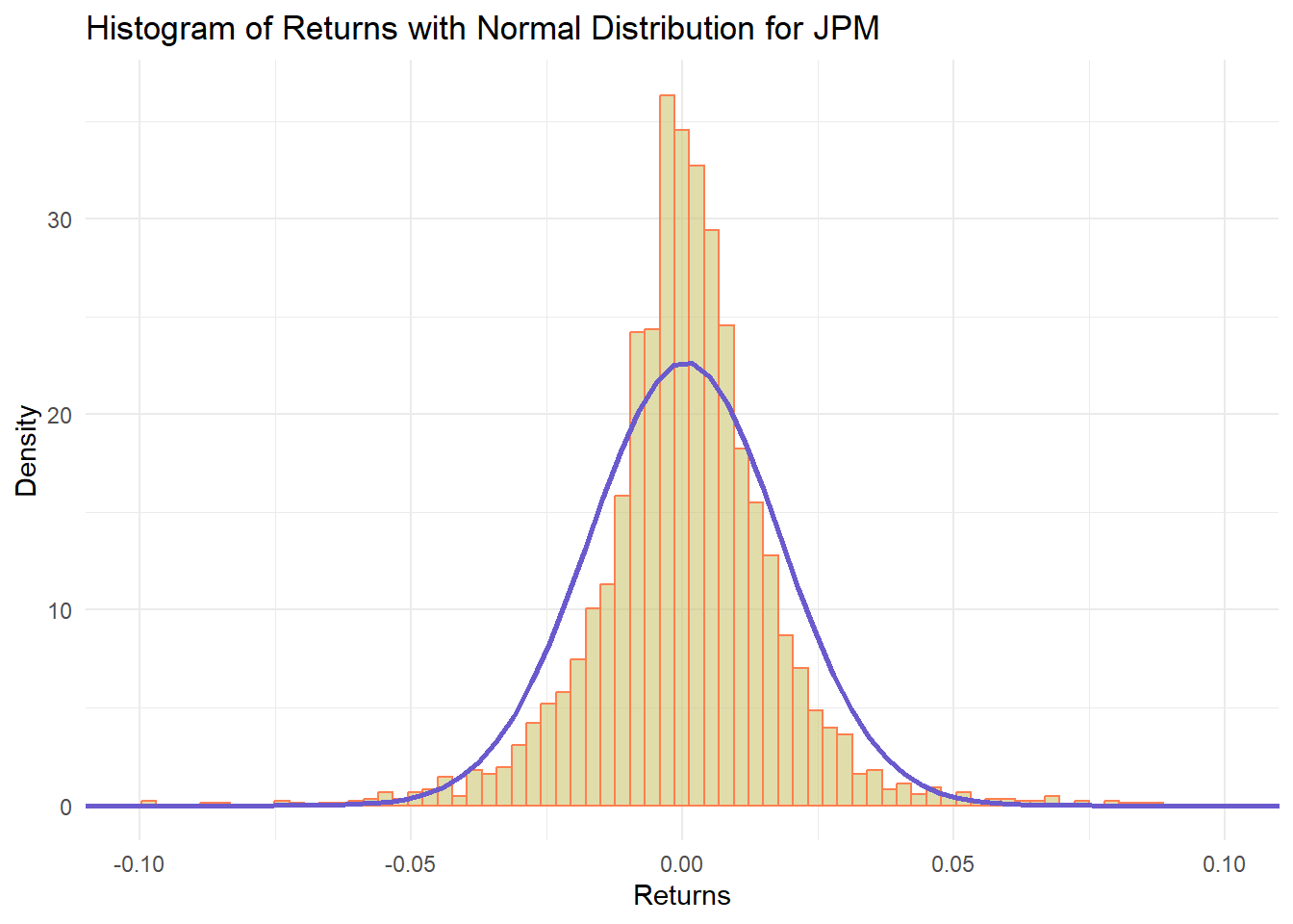
pg_hist_plot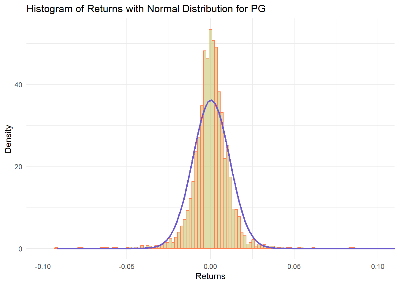
nvda_hist_plot
Summarize the moments
# Function to calculate the summary statistics
calculate_stats <- function(data, return_col) {
    data |>
        summarize(
            mean = mean({{ return_col }}, na.rm = TRUE),
            sd = sd({{ return_col }}, na.rm = TRUE),
            skew = skewness({{ return_col }}, na.rm = TRUE),
            kurt = kurtosis({{ return_col }}, na.rm = TRUE)
            )
}


# Calculate statistics for each stock and store them in a tibble
stats_tibble <- tibble(
    stock = c("PG", "JPM", "NVDA"),
    stats = list(
        calculate_stats(pg_data, daily.returns),
        calculate_stats(jpm_data, daily.returns),
        calculate_stats(nvda_data, daily.returns)
        )
    )

# Unnest the stats column to expand the tibble
stats_tibble <- stats_tibble |>
    unnest(stats)

stats_tibble |> gt() |>
    fmt_percent(columns = vars(mean, sd), decimals = 4) |>
    fmt_number(columns = vars(skew, kurt), decimals = 4) |>
    data_color(
        columns = 4,
        domain = c(-0.2, 0.4),
        palette = c("lightpink", "seagreen1"),
        alpha = 0.5
    ) |>
    data_color(
        columns = 5,
        domain = c(0, 15),
        palette = c("lightpink", "seagreen1"),
        alpha = 0.5
)| stock | mean | sd | skew | kurt |
|---|---|---|---|---|
| PG | 0.0380% | 1.1017% | −0.0216 | 14.7342 |
| JPM | 0.0490% | 1.7601% | −0.0967 | 13.3437 |
| NVDA | 0.1509% | 2.8227% | 0.2871 | 10.6039 |
For fun (the social thumb)
nvda_roll_plot / garch_p1