Value at Risk (VaR) Introduction

Contents

• Historical Simulation: Basic and Bootstrap
• Monte Carlo
• Parametric; aka, analytical

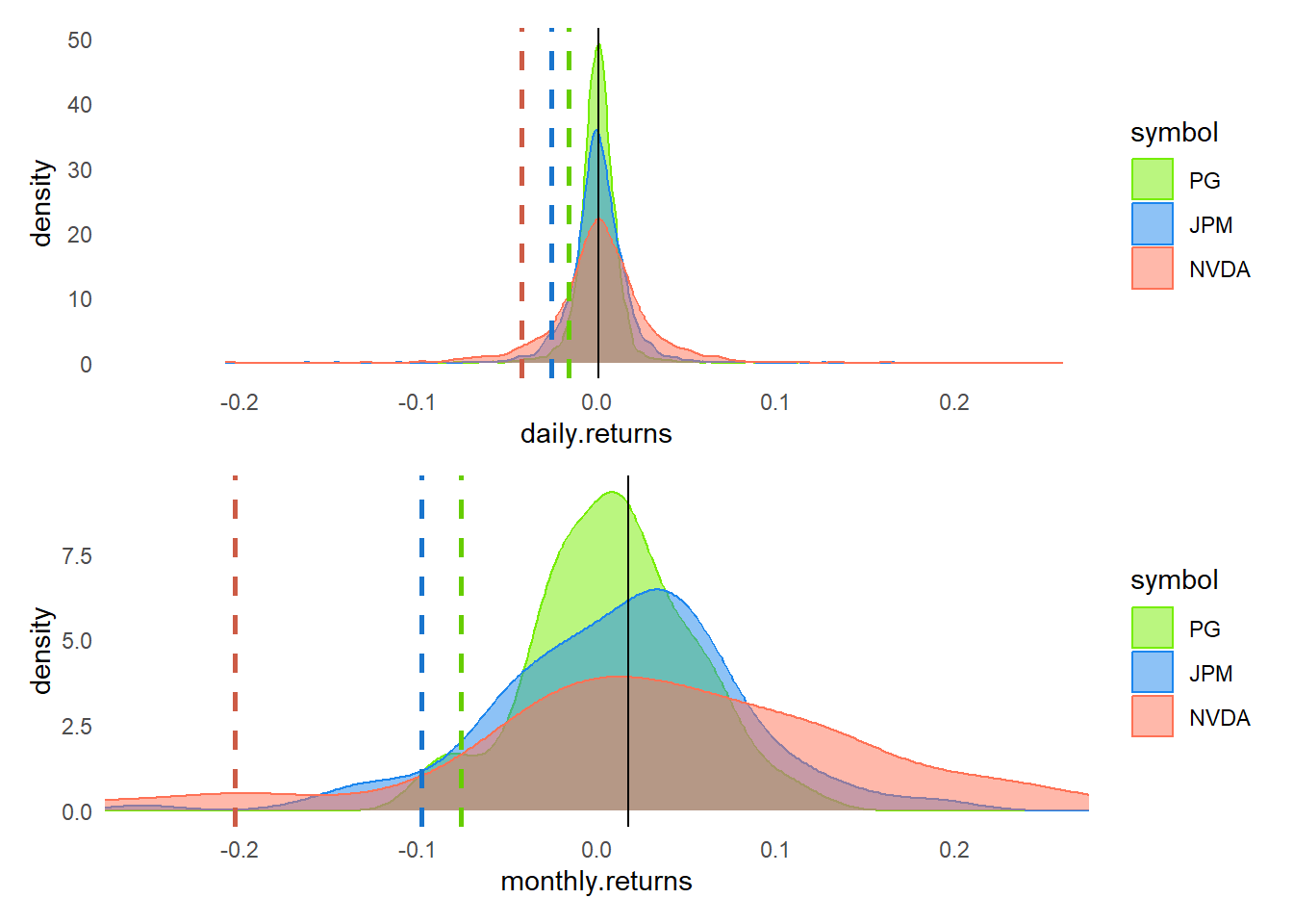
Historical simulation (HS)

Basic HS

library(tidyverse)
library(tidyquant)
library(patchwork)
library(scales)

symbols <- c("PG", "JPM", "NVDA")
mult_stocks <- tq_get(symbols, get = "stock.prices", from = "2012-12-31", to = "2022-12-31")
mult_stocks$symbol <- mult_stocks$symbol <- factor(mult_stocks$symbol, levels = c("PG", "JPM", "NVDA"))

# tq_mutate_fun_options() returns list of compatible mutate functions by pkg 
all_returns_daily <- mult_stocks |> 
    group_by(symbol) |>
    tq_transmute(select     = adjusted,
                 mutate_fun = periodReturn, 
                 period     = "daily", 
                 type       = "log")

all_returns_monthly <- mult_stocks |> 
    group_by(symbol) |> 
    tq_transmute(select     = adjusted, 
                 mutate_fun = periodReturn, 
                 period     = "monthly",
                 type       = "log")

# reframe() has apparently replaced summarize()
quantiles_daily <- all_returns_daily |> 
    group_by(symbol) |> 
    reframe(quantiles = quantile(daily.returns, probs = c(0.05, 0.95)))

quantiles_monthly <- all_returns_monthly |> 
    group_by(symbol) |> 
    reframe(quantiles = quantile(monthly.returns, probs = c(0.05, 0.95)))

# 5% quantile for each stock, DAILY
PG_05d <- quantiles_daily$quantiles[1]
JPM_05d <- quantiles_daily$quantiles[3]
NVDA_05d <- quantiles_daily$quantiles[5]
mean_d <- mean(all_returns_daily$daily.returns) 

# 5% quantile for each stock, MONTHLY
PG_05m <- quantiles_monthly$quantiles[1]
JPM_05m <- quantiles_monthly$quantiles[3]
NVDA_05m <- quantiles_monthly$quantiles[5]
mean_m <- mean(all_returns_monthly$monthly.returns)

# I probably spend too much time tinkering with colors
# col_ticker_fills <- c("PG" = "blue", "JPM" = "yellow", "NVDA" = "red")
# col_ticker_fills <- c("PG" = "#90EE90", "JPM" = "#ff6347", "NVDA" = "#8B0000")
col_ticker_fills <- c("PG" = "chartreuse2", "JPM" = "dodgerblue2", "NVDA" = "coral1")
col_ticker_colors <- c("PG" = "chartreuse3", "JPM" = "dodgerblue3", "NVDA" = "coral3")
col_PG_line <- "chartreuse3"; col_JPM_line <- "dodgerblue3"; col_NVDA_line <- "coral3"

p_hist_daily <- all_returns_daily |> 
    ggplot(aes(x = daily.returns, fill = symbol, color = symbol)) +
    geom_density(alpha = 0.50) +
    geom_vline(xintercept = PG_05d, color = col_PG_line, linetype = "dashed", linewidth = 1) +
    geom_vline(xintercept = JPM_05d, color = col_JPM_line, linetype = "dashed", linewidth = 1) + 
    geom_vline(xintercept = NVDA_05d, color = col_NVDA_line, linetype = "dashed", linewidth = 1) +
    geom_vline(xintercept = mean_d, color = "black", linewidth = 0.4) +
    scale_fill_manual(values = col_ticker_fills) +
    scale_color_manual(values = col_ticker_fills) +
    theme_minimal() +
    coord_cartesian(xlim = c(-0.25, 0.25)) +
        theme(
        panel.grid.major = element_blank(),
        panel.grid.minor = element_blank(),
    )

p_hist_monthly <- all_returns_monthly |> 
    ggplot(aes(x = monthly.returns, fill = symbol, color = symbol)) +
    geom_density(alpha = 0.50) +
    geom_vline(xintercept = PG_05m, color = col_PG_line, linetype = "dashed", linewidth = 1) +
    geom_vline(xintercept = JPM_05m, color = col_JPM_line, linetype = "dashed", linewidth = 1) + 
    geom_vline(xintercept = NVDA_05m, color = col_NVDA_line, linetype = "dashed", linewidth = 1) +
    geom_vline(xintercept = mean_m, color = "black", linewidth = 0.4) +
    scale_fill_manual(values = col_ticker_fills) +
    scale_color_manual(values = col_ticker_fills) +
    theme_minimal() + 
    coord_cartesian(xlim = c(-0.25, 0.25)) +
    theme(
        panel.grid.major = element_blank(),
        panel.grid.minor = element_blank(),
    )

p_hs <- p_hist_daily / p_hist_monthly
p_hs

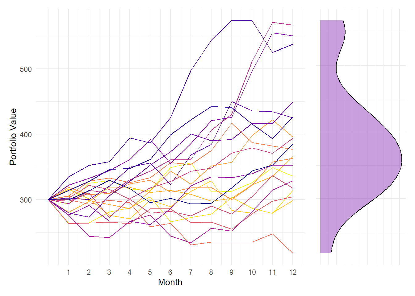
Bootstrap HS

First let’s simulate a single one-year forward (+ 12 months) path

# all_returns_monthly is tidy, but the simulation wants a wide format
all_returns_monthly_wide <- all_returns_monthly |> 
  pivot_wider(names_from = symbol, values_from = monthly.returns)

# Initial investment (into each stock)
initial_investment <- 100
portfolio <- setNames(data.frame(t(rep(initial_investment, times = length(symbols)))), symbols)
months_to_simulate <- 12 # Set X months for the simulation

# Simulate one forward month
simulate_one_month <- function(portfolio, historical_returns_wide) {
    # Randomly sample one month's returns (with replacement)
    sampled_returns <- historical_returns_wide |>  
        sample_n(1, replace = TRUE) |> select(-date) 
    # Apply the sampled log returns to the current portfolio value
    updated_portfolio <- portfolio * exp(sampled_returns)
    # FOR TESTING: print(sampled_returns[1,]); print(updated_portfolio[1,])
    return(updated_portfolio)
}

# Run the simulation for X months
set.seed(123) # For reproducibility of results
simulation_results <- tibble(Month = 0, TotalValue = sum(portfolio))
for (i in 1:months_to_simulate) {
    portfolio <- simulate_one_month(portfolio, all_returns_monthly_wide)
    simulation_results <- simulation_results |>  
        add_row(Month = i, TotalValue = sum(portfolio))
}

print(simulation_results)

# A tibble: 13 × 2
   Month TotalValue
   <dbl>      <dbl>
 1     0       300 
 2     1       294.
 3     2       325.
 4     3       329.
 5     4       316.
 6     5       314.
 7     6       349.
 8     7       356.
 9     8       312.
10     9       313.
11    10       326.
12    11       349.
13    12       336.

Next let’s add a loop to run the simulation multiple times; e.g. 20 trials

library(RColorBrewer)
# library(ggside) couldn't pull it off! 

# Function to simulate portfolio over X months, where each trail has a trial_id
simulate_portfolio <- function(months_to_simulate, historical_returns_wide, initial_investment, trial_id) {
    # Initialize portfolio
    portfolio <- setNames(data.frame(t(rep(initial_investment, times = length(symbols)))), symbols)
    # Initialize results data frame with Month 0
    simulation_results <- tibble(Month = 0, TotalValue = sum(portfolio), Trial = as.factor(trial_id))
    for (i in 1:months_to_simulate) {
        portfolio <- simulate_one_month(portfolio, historical_returns_wide)
        simulation_results <- simulation_results |> 
            add_row(Month = i, TotalValue = sum(portfolio), Trial = as.factor(trial_id))
    }
  return(simulation_results)
}

months_to_simulate <- 12 
num_trials <- 20 # Number of trials

set.seed(123) 
all_trials <- map_df(1:num_trials, 
                     ~simulate_portfolio(months_to_simulate, all_returns_monthly_wide, initial_investment, .x), 
                     .id = "Trial_ID")

final_month_values_df <- all_trials |> 
    filter(Month == max(all_trials$Month))

# Plot the results using ggplot2
p_forward_sim <- ggplot(all_trials, aes(x = Month, y = TotalValue, group = Trial, color = Trial)) +
    geom_line() +
    scale_color_viridis_d(option = "plasma", direction = -1) +
    theme_minimal() +
    scale_x_continuous(breaks = 1:12, limits = c(0,12)) +
    labs(x = "Month",
         y = "Portfolio Value") +
    theme(legend.position = "none") 

density_plot <- final_month_values_df |> ggplot(aes(x = TotalValue)) +
    geom_density(fill = "#933fbd", alpha = 0.5) +
        theme_minimal() + 
    theme(
        axis.title = element_blank(),
        axis.text = element_blank()
    ) +
    coord_flip()

p_boot <- p_forward_sim + density_plot + 
    plot_layout(ncol = 2, widths = c(3, 1))
p_boot

final_month_values_vct <- final_month_values_df |> 
    pull(TotalValue) # 'pull' extracts the column as a vector

# Calculate and print the quantiles for the final month's values
quantiles_final_month <- quantile(final_month_values_vct, probs = c(0, 0.01, 0.05, 0.50, 1.0))
print(quantiles_final_month)

      0%       1%       5%      50%     100% 
218.1581 233.4910 294.8226 371.7791 567.0854 

Monte carlos simulation (MCS)

First a single path:

sim_gbm <- function(price, mu, sigma, periods) {
  dt <- 1/52  # we'll assume period is one week
  prices <- numeric(periods)
  prices[1] <- price

    for(t in 2:periods) {
    Z <- rnorm(1) # random standar normal quantile
    
    # GBM
    prices[t] <- prices[t-1]*exp((mu -0.5*sigma^2)*dt +sigma*sqrt(dt)*Z)
    }
  return(prices)
}

set.seed(952347)
sim_prices <- sim_gbm(100, 0.09, 0.3, 50)
sim_prices_df <- as_tibble(sim_prices) |> rownames_to_column("period")
sim_prices_df$period <- as.integer(sim_prices_df$period)

# Plot the simulated stock price path
sim_prices_df |> 
    ggplot(aes(x = period, y = value)) + 
    geom_line() + 
    theme_minimal() 

Now multiple (say 20) trials:

sim_gbm_matrix <- function(price, mu, sigma, periods, simulations) {
  dt <- 1/52  
  prices <- matrix(price, nrow = periods, ncol = simulations)
  for(t in 2:periods) {
    Z <- rnorm(simulations)
    prices[t, ] <- prices[t-1, ] * exp((mu - 0.5 * sigma^2) * dt + sigma * sqrt(dt) * Z)
  }
  return(prices)
}

set.seed(84923)
simulations <- 20
sim_prices_matrix <- sim_gbm_matrix(100, 0.09, 0.3, 50, simulations)

sim_prices_df <- as_tibble(sim_prices_matrix, .name_repair = "minimal")
names(sim_prices_df) <- 1:ncol(sim_prices_df)
sim_prices_df <- sim_prices_df |> rownames_to_column("period")
sim_prices_df$period <- as.integer(sim_prices_df$period)

sim_prices_long <- sim_prices_df |> 
  pivot_longer(cols = !period, names_to = "Trial", values_to = "Price")

p_mcs <- sim_prices_long |> ggplot(aes(x = period, y = Price, group = Trial, color = Trial)) +
    geom_line() +
    labs(x = "Week",
         y = "Price") +
    theme_minimal() +
    theme(
        legend.position = "none"
    ) +
    scale_color_viridis_d()

p_mcs + ggtitle("GBM MCS: 20 trials x 50 weeks")

Parametric: normally distributed arithmetic returns

The basic starting point: normal, arithmetic returns and scaling per the square root rule (SRR) which asumes i.i.d. returns.

library(ggplot2)

# Parameters
mu_pa <- 0.09
sigma_pa <- 0.20
horizon <- 12/52

mu <- mu_pa * horizon  # horizon return
sigma <- sigma_pa * sqrt(horizon)  # horizon volatility
confidence_level <- 0.95
investment_value <- 100  # Initial investment

# Find the Z-score that corresponds to the confidence level
z_score <- qnorm(confidence_level)
VaR <- (-mu + sigma * z_score) * investment_value

# Create a dataframe of returns for plotting
returns <- data.frame(Returns = seq(-0.30, 0.30, by = 0.001))
returns$Density <- dnorm(returns$Returns, mean = mu, sd = sigma)

# Plot with ggplot
p_pVaR <- ggplot(returns, aes(x = Returns, y = Density)) +
    geom_line(color = "dodgerblue", linewidth = 1.3) +
    geom_vline(xintercept = -VaR / investment_value, color = "darkred", linetype = "dashed", linewidth = 1.3) +
    geom_area(data = subset(returns, Returns < -VaR / investment_value),
              aes(x = Returns, y = Density), fill = "coral1", alpha = 0.5) +
    geom_vline(xintercept = mu, color = "chartreuse3", linetype = "dashed", linewidth = 1.3) + 
    geom_vline(xintercept = 0, color = "black", linewidth = 0.4) +
    scale_x_continuous(labels = percent_format(),
                       breaks = seq(-0.30, 0.30, by = 0.1)) +
    theme_minimal() +
    theme(
        panel.grid.major.y = element_blank(),
        panel.grid.minor.y = element_blank(),
        axis.title.y = element_blank(),
        axis.text.y = element_blank()
    ) + 
    annotate("text", x = -VaR / investment_value + .02, 
             y = max(returns$Density)/3,
             label = paste("VaR at", scales::percent(confidence_level), "=", round(VaR, 3)),
             hjust = 1.2, vjust = 0, size = 4, color = "darkred", fontface = "bold")

p_pVaR + ggtitle("Normal, arithmetic i.i.d. returns")

For fun: Using patchwork to print the social thumbnail!

# layout <- "
# AABBCC
# AABBCC
# DDDDEE
# DDDDEE
# "
# 
# p_hs + p_pVaR + p_boot + p_mcs +
#    plot_layout(design = layout)

p_hs / p_boot / (p_mcs + p_pVaR)