finedtech by David Harper, CFA, FRM

Contents

Visualizing nearest neighbors in two-dimensional feature space (simulated borrow default based on credit score and income)
Parallel coordinates plot to visualize nearest neighbors in multi-dimensional feature space (Wisconsin breast cancer dataset with 30 features)

First the libraries:

my_libraries <- c("tidyverse", "ggforce", "janitor", "openxlsx", "patchwork", # for mine
                  "class", "GGally", "viridis") # for Lantz's data
lapply(my_libraries, library, character.only = TRUE)

library(class)
library(GGally)
library(viridis)

Predicting loan default based on vote of nearest neighbors

Because it’s easy to visualize, my first example is simulated data in a two-dimensional feature space. The training set is 100 borrowers with credit scores and incomes. This is supervised learning: the borrowers either defaulted or repaid. The single test point (see blue triangle below) is a borrower with a credit score of 605 and income of $41,000.

set.seed(743) 
n <- 100 

credit_scores <- rnorm(n, mean=650, sd=50)
incomes <- rnorm(n, mean=50000, sd=10000)

# Default if credit score is below 600 OR income is below $40,000
labels <- ifelse(credit_scores < 600 | incomes < 40000, "default", "repay")

# But switch some "repay" to "default" to add noise
random_indices <- sample(1:n, n/10) # Arbitrary 10%
labels[random_indices] <- "default"

train <- data.frame(credit_score=credit_scores, income=incomes, label=labels)
# In k-nn, we should either standardize or normalize the data
mu_credit <- mean(train$credit_score); sig_credit <- sd(train$credit_score)
mu_income <- mean(train$income); sig_income <- sd(train$income)
train$credit_score_std <- (train$credit_score - mu_credit) / sig_credit
train$income_std <- (train$income - mu_income) / sig_income

# The test point; then standardized
x <- 605
y <- 41000
x_std <- (x - mu_credit) / sig_credit
y_std <- (y - mu_income) / sig_income

# Euclidean distance (from all points) to test point
distances_std <- sqrt((train$credit_score_std - x_std)^2 + (train$income_std - y_std)^2)

# The k-nearest neighbors are simply the k (=5 or =10 or =15, eg) smallest distances
k05 <- 5; k10 <- 10; k15 <- 15

k_nearest_indices_std_05 <- order(distances_std)[1:k05]
k_nearest_indices_std_10 <- order(distances_std)[1:k10]
k_nearest_indices_std_15 <- order(distances_std)[1:k15]

# Add distances column and display  k-nearest neighbors with their distance
k_nn <- train[k_nearest_indices_std_15, ]
nearest <- distances_std[k_nearest_indices_std_15]
k_nn$distance <- nearest

# k_nearest_neighbors
k_nn |> adorn_rounding(digits = 0, rounding = "half up", 
                                      all_of(c("credit_score", "income"))) |> 
    adorn_rounding(digits = 3, rounding = "half up", credit_score_std:distance)

   credit_score income   label credit_score_std income_std distance
8           611  41988   repay           -0.804     -0.759    0.145
82          598  39398 default           -1.035     -1.016    0.201
41          603  43184   repay           -0.951     -0.641    0.220
4           592  39166 default           -1.150     -1.039    0.300
64          604  44168   repay           -0.932     -0.543    0.315
32          587  41994 default           -1.243     -0.759    0.345
75          621  44367   repay           -0.618     -0.523    0.445
53          627  38749 default           -0.513     -1.081    0.457
1           583  46197 default           -1.307     -0.342    0.650
45          598  34567 default           -1.045     -1.496    0.652
11          639  43148   repay           -0.282     -0.644    0.665
80          640  43630   repay           -0.263     -0.596    0.699
84          643  43094   repay           -0.219     -0.650    0.723
52          646  41064   repay           -0.156     -0.851    0.756
99          639  45497   repay           -0.295     -0.411    0.761

# Now the ggplots!
# colors
three_colors <- c("default" = "lightpink1", "repay" = "lightgreen")
five_colors <- c("default" = "lightpink1", "repay" = "lightgreen", "NN Default" = "red", "NN Repay" = "green4")    

# Base plots, with labels and without (and zoomed in per coord_cartesian)
p_base_lab <- ggplot(train, aes(x=credit_score_std, y=income_std)) +
    geom_point(aes(x=x_std, y=y_std), color="dodgerblue2", shape=17, size=4) +
    xlab("Credit Score (Standardized)") +
    ylab("Income (Standardized)") +
    theme_minimal()

p_base <- ggplot(train, aes(x=credit_score_std, y=income_std)) + 
    geom_point(aes(x=x_std, y=y_std), color="dodgerblue2", shape=17, size=4) +
    theme_minimal() +
    theme(legend.position = "none", axis.title = element_blank()) +
    coord_cartesian(xlim = c(-1.75, 0), ylim = c(-1.75, 0))

p1_lab <- p_base_lab + 
    geom_point(aes(color = label), size = 3) + 
    labs(title = paste("The majority of how many k neighbors?"),
         subtitle = paste("Blue triangle is Test point"),
         color = "Borrower") +
    scale_color_manual(values = three_colors)

p3_lab <- p_base_lab +
    geom_point(aes(color = ifelse(row.names(train) %in% row.names(train[k_nearest_indices_std_10, ]),
                                  ifelse(label == "default", "NN Default", "NN Repay"),
                                  label)), size = 3) +
    labs(title = paste("Let's ask k = 10 neighbors to vote"),
         subtitle = paste("Six defaulted and four repaid (radius is ~0.652)"),
         color = "Borrower") +
    geom_circle(aes(x0 = x_std, y0 = y_std, r = 0.658), 
              color = "blue",linetype="dashed", fill = NA) +
    scale_color_manual(values = five_colors)

p1_lab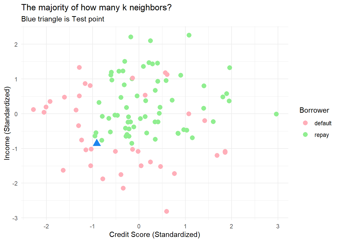

p3_lab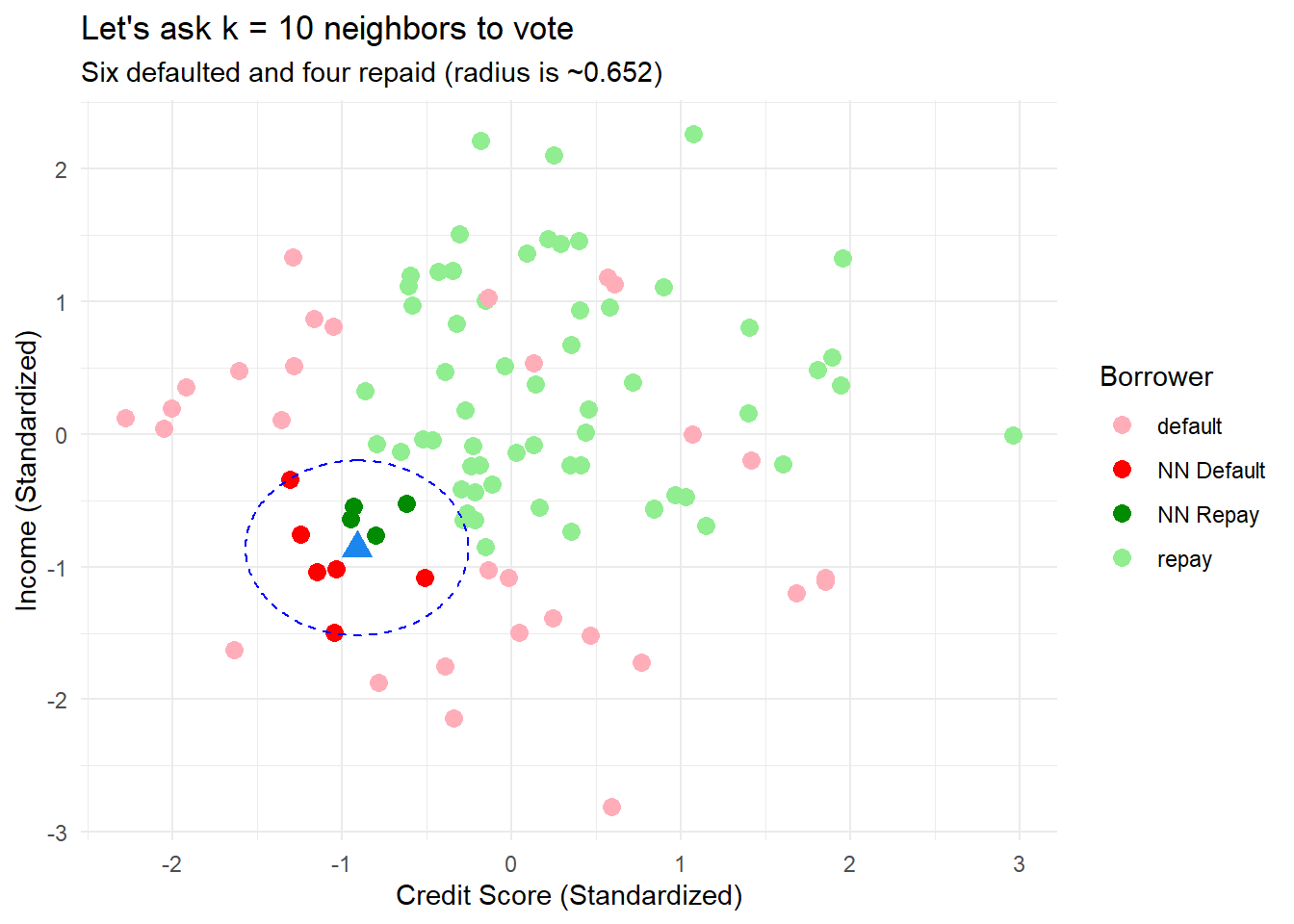

p1 <- p_base + 
    geom_point(aes(color = label), size = 3) +
    scale_color_manual(values = three_colors)

p2 <- p_base + 
    geom_point(aes(color = ifelse(row.names(train) %in% row.names(train[k_nearest_indices_std_05, ]),
                                  ifelse(label == "default", "NN Default", "NN Repay"),
                                  label)), size = 3) +
    geom_circle(aes(x0 = x_std, y0 = y_std, r = 0.330), 
              color = "blue",linetype="dashed", fill = NA) +
    scale_color_manual(values = five_colors) 

 p3 <- p_base +
    geom_point(aes(color = ifelse(row.names(train) %in% row.names(train[k_nearest_indices_std_10, ]),
                                  ifelse(label == "default", "NN Default", "NN Repay"),
                                  label)), size = 3) +
    geom_circle(aes(x0 = x_std, y0 = y_std, r = 0.658), 
              color = "blue",linetype="dashed", fill = NA) +
    scale_color_manual(values = five_colors)

 p4 <- p_base +
    geom_point(aes(color = ifelse(row.names(train) %in% row.names(train[k_nearest_indices_std_15, ]),
                                  ifelse(label == "default", "NN Default", "NN Repay"),
                                  label)), size = 3) +
     geom_circle(aes(x0 = x_std, y0 = y_std, r = 0.763), 
              color = "blue",linetype="dashed", fill = NA) +
    scale_color_manual(values = five_colors) 

(p1 | p2) / (p3 | p4) + 
     plot_annotation(title = "Top: None and k = 5, Bottom: k = 10 and k = 15", 
                     subtitle = "From repay (3/5) to default (6/10) to repay (9/15)")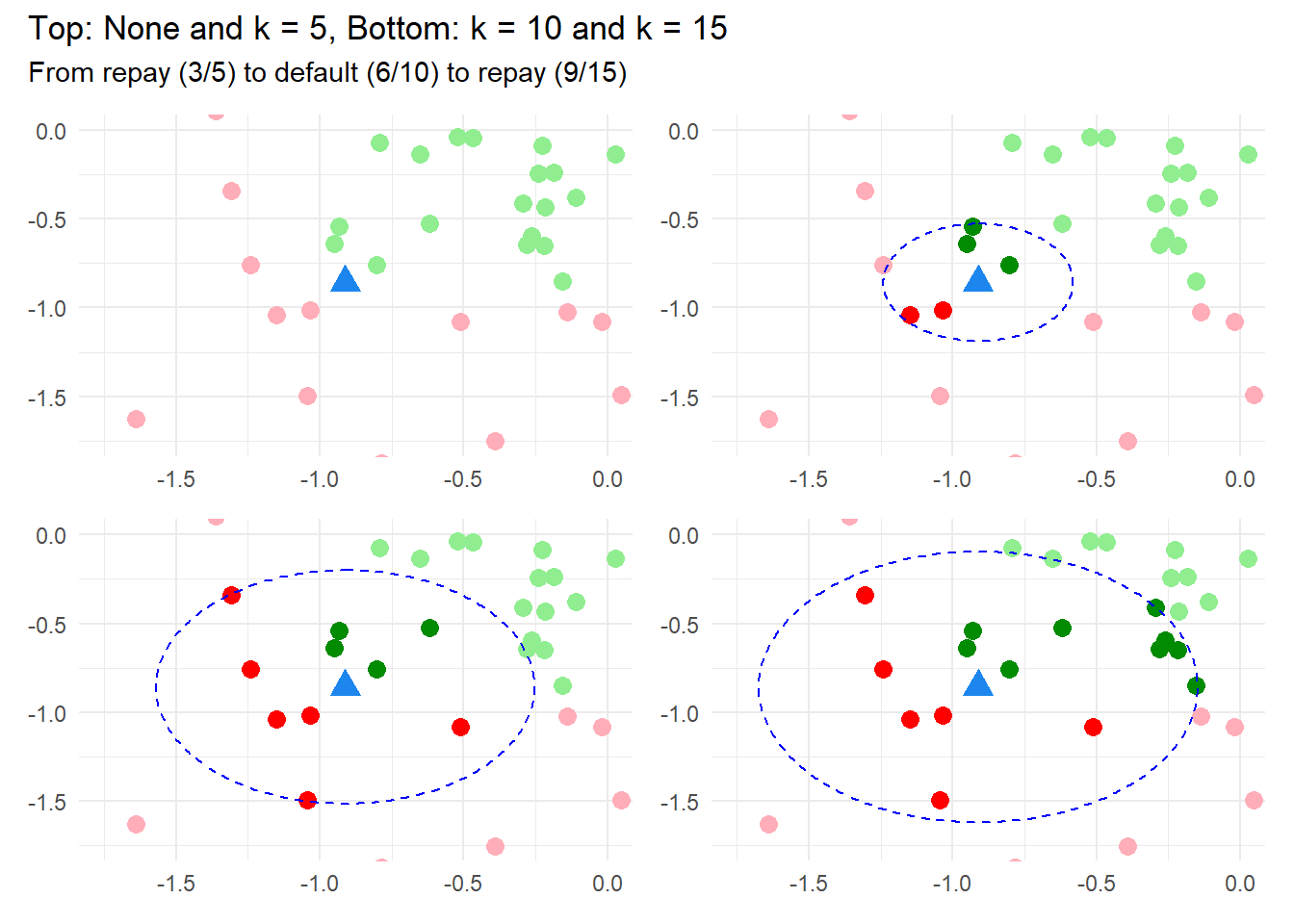

Predicting default based on vote of nearest neighbors

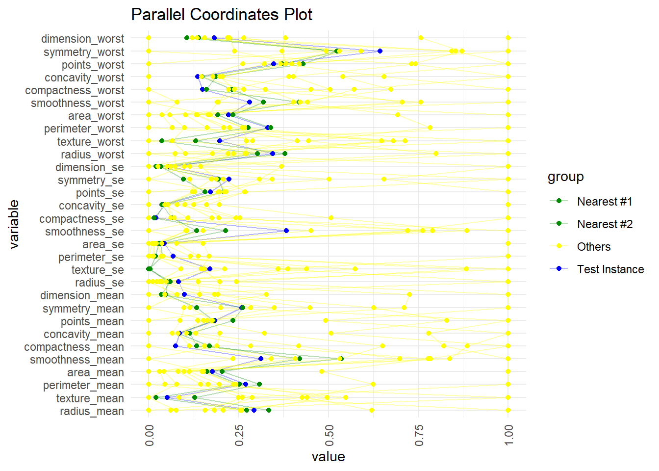
Most datasets have many features. I quickly tried a few experiments to visualize multidimensional neighbors. At this point, my favorite is the parallel coordinates plot below. I’ll use the dataset from my favorite machine learning introduction: Machine Learning with R by Brent Lantz, 4th Edition. He did not attempt to visualize this nearest neighbor’s example.

We’re using the Wisconsin Breast Cancer Dataset. The dataset has 569 observations and 30 numeric features that describe characteristics of the cell nuclei present in the image. The target variable is the diagnosis (benign or malignant).

Brett Lantz parses the dataset into 469 training observation and 100 test observations. Please note that these features are normalized (i.e., on a zero to one scale) rather than standardized (as I did above). Below, I retrieve the first test instance and plot its two nearest (Euclidean) neighbors in the training set. Although this does not convey numerical distance (obviously), I think it’s a fine way to illustrate the proximity of the features.

load("wbcd_dfs.RData") # wbcd_train, wbcd_train_labels, wbcd_test, wbcd_test_labels
# I previously retrieved the nearest neighbors to the single test instance
# k_nearest neighbors <- function(test_instance, train_data, k)
# save(k_neighbors, file = "k_neighbors.RData")
load("k_neighbors.RData") # k_neighbors

str(wbcd_train)

'data.frame':   469 obs. of  30 variables:
 $ radius_mean      : num  0.253 0.171 0.192 0.203 0.389 ...
 $ texture_mean     : num  0.0906 0.3125 0.2408 0.1245 0.1184 ...
 $ perimeter_mean   : num  0.242 0.176 0.187 0.202 0.372 ...
 $ area_mean        : num  0.136 0.0861 0.0974 0.1024 0.2411 ...
 $ smoothness_mean  : num  0.453 0.399 0.497 0.576 0.244 ...
 $ compactness_mean : num  0.155 0.292 0.18 0.289 0.153 ...
 $ concavity_mean   : num  0.0934 0.1496 0.0714 0.1086 0.0795 ...
 $ points_mean      : num  0.184 0.131 0.123 0.238 0.132 ...
 $ symmetry_mean    : num  0.454 0.435 0.33 0.359 0.334 ...
 $ dimension_mean   : num  0.202 0.315 0.283 0.227 0.115 ...
 $ radius_se        : num  0.0451 0.1228 0.0309 0.0822 0.0242 ...
 $ texture_se       : num  0.0675 0.1849 0.2269 0.2172 0.0116 ...
 $ perimeter_se     : num  0.043 0.1259 0.0276 0.0515 0.0274 ...
 $ area_se          : num  0.0199 0.0379 0.0126 0.0365 0.0204 ...
 $ smoothness_se    : num  0.215 0.196 0.117 0.325 0.112 ...
 $ compactness_se   : num  0.0717 0.252 0.0533 0.2458 0.0946 ...
 $ concavity_se     : num  0.0425 0.0847 0.0267 0.0552 0.0392 ...
 $ points_se        : num  0.235 0.259 0.142 0.372 0.173 ...
 $ symmetry_se      : num  0.16 0.382 0.131 0.111 0.121 ...
 $ dimension_se     : num  0.0468 0.0837 0.045 0.088 0.0301 ...
 $ radius_worst     : num  0.198 0.141 0.159 0.142 0.294 ...
 $ texture_worst    : num  0.0965 0.291 0.3843 0.0999 0.0989 ...
 $ perimeter_worst  : num  0.182 0.139 0.147 0.13 0.269 ...
 $ area_worst       : num  0.0894 0.0589 0.0703 0.0611 0.1558 ...
 $ smoothness_worst : num  0.445 0.331 0.434 0.433 0.274 ...
 $ compactness_worst: num  0.0964 0.2175 0.1173 0.1503 0.142 ...
 $ concavity_worst  : num  0.0992 0.153 0.0852 0.0692 0.1088 ...
 $ points_worst     : num  0.323 0.272 0.255 0.296 0.281 ...
 $ symmetry_worst   : num  0.249 0.271 0.282 0.106 0.182 ...
 $ dimension_worst  : num  0.0831 0.1366 0.1559 0.084 0.0828 ...

# this knn() function is from the class package
# and it classifies the test set; e.g., 1st is classified as Benign
wbcd_test_pred <- knn(train = wbcd_train, test = wbcd_test,
                      cl = wbcd_train_labels, k = 21)
wbcd_test_pred[1]

[1] Benign
Levels: Benign Malignant

# inserting first instance at top of training set for graph
wbcd_train <- rbind(wbcd_test[1, ], wbcd_train) # 469 + 1 = 470

wbcd_train$group <- "Others"
wbcd_train$group[1] <- "Test Instance"
obs_2_index <- k_neighbors[1] + 1
wbcd_train$group[obs_2_index] <- "Nearest #1"
obs_3_index <- k_neighbors[2] + 1
wbcd_train$group[obs_3_index] <- "Nearest #2"

# set.seed(479)
set.seed(48514)

# Set the row indices you want to include
row1 <- 1
row2 <- obs_2_index
row3 <- obs_3_index

# Number of random rows to sample
n <- 10

# Sample without the specific rows, then combine with the specific rows
sampled_indices <- sample(setdiff(1:nrow(wbcd_train), c(row1, row2, row3)), n)
final_sample <- rbind(wbcd_train[c(row1, row2, row3), ], wbcd_train[sampled_indices, ])

final_sample |> ggparcoord(columns = 1:30, 
                           groupColumn = "group",
                           showPoints = TRUE,
                           alphaLines = 0.3,
                           scale = "uniminmax") +
    scale_color_manual(values = c("Test Instance" = "blue",
                                  "Nearest #1" = "green4",
                                  "Nearest #2" = "green4",
                                  "Others" = "yellow")) + 
    theme_minimal() +
    labs(title = "Parallel Coordinates Plot") +
    theme(axis.text.x = element_text(angle = 90, vjust = 0.5, hjust=1)) +
    coord_flip()