Logistic regression

Simulated insurance dataset (via simdata) and visualization of marginal effects (via ggeffects)
code
analysis
Author

David Harper, CFA, FRM

Published

October 29, 2023

Simulate data with simdata package

The delightful simdata package allows us to specify a correlation matrix and tranform (via transformation function) the random multivarate normal distribution into the set of desired univariate (but correlated!) distributions.

library(tidyverse)
library(gt)

library(patchwork)
library(GGally); library(ggcorrplot)
library(ggeffects) # amazing package plots marginal effects

library(simdata)
library(matrixcalc); library(mbend)
library(gmodels) # CrossTable()

library(skimr)

# this function in the simdata package builds a correlation
# matrix by specifying c(col, row, rho)
correlation_matrix = cor_from_upper(
    8,
    rbind(c(1,8,-0.20), # loyalty
          c(2,8,-0.16), # bundle
          c(3,8,0.12),  # jump (in price)
          c(4,8,0.15),  # premium
          c(5,8,-0.07), # age
          c(6,8,-0.05), # income
          c(7,8,0))     # mobile
)

# we require positive definite matrix
# is.positive.definite(correlation_matrix) = TRUE
if (!is.positive.definite(correlation_matrix)) {
    correlation_matrix <- bend(correlation_matrix)$bent |> round(5)
}

ggcorrplot(correlation_matrix,
           colors = c("red","white", "darkgreen"))

transformation <- simdata::function_list(
    loyalty = function(z) qbeta(pnorm(z[,1]), shape1 = 2, shape2 = 5) * 30,
    bundle_b = function(z) z[,2] > qnorm(0.7), #bundle
    pricejump_b = function(z) z[,3] > qnorm(0.8),  # 80th for 20% probability
    premium = function(z) pnorm(z[,4]) * (2000 - 300) + 300, # premium
    age = function(z) pmax(18, pmin(80, z[,5] * 10 + 40)), #age
    income = function(z) exp(z[,6] + 4), #income
    mobile_b = function(z) z[,7] > 0, #mobile
    churn = function(z) z[,8] > qnorm(.8)
)

# the multivarate normal design specification
sim_design = simdata::simdesign_mvtnorm(
  relations = correlation_matrix,
  transform_initial = transformation,
  prefix_final = NULL
)

sim_data = simdata::simulate_data(sim_design, n_obs = 1000, seed = 51493)

sim_data$churn <- as.factor(sim_data$churn)
sim_data$loyalty <- round(sim_data$loyalty, 1)
sim_data$bundle_b <- as.factor(sim_data$bundle_b) #ok
sim_data$pricejump_b <- as.factor(sim_data$pricejump_b) #ok
sim_data$premium <- round(sim_data$premium/10)*10
sim_data$age <- round(sim_data$age)
sim_data$income <- round(sim_data$income/10)*10
sim_data$mobile_b <- as.factor(sim_data$mobile_b) #ok

# don't use v1, instead will split into train/test sets
# model_sim_v1 <- glm(formula = churn ~ .,
#        family = binomial(link = "logit"), data = sim_data)
# summary(model_sim_v1)

set.seed(7553695)
train_sample <- sample(1000, 900)
sim_train <- sim_data[train_sample, ]
sim_test <- sim_data[-train_sample, ]

data_scenario_range <- data.frame(
    loyalty = c(25,20,15,10,5,1),
    bundle_b = as.factor(c(TRUE,TRUE,TRUE,FALSE,FALSE,FALSE)),
    pricejump_b = as.factor(c(FALSE,FALSE,FALSE,FALSE,TRUE,TRUE)),
    premium = c(300,500,900,1100,1600,2000),
    age = c(70,55,40,29,24,21),
    income = c(200,150,120,100,80,60),
    mobile_b = as.factor(c(TRUE,FALSE,TRUE,FALSE,TRUE,FALSE))
)

data_feature_means <- data.frame(
    loyalty = mean(sim_train$loyalty),
    bundle_b = as.factor(FALSE),
    pricejump_b = as.factor(FALSE),
    premium = mean(sim_train$premium),
    age = mean(sim_train$age),
    income = mean(sim_train$income),
    mobile_b = as.factor(TRUE)
)

ggpairs(sim_train, columns = 1:6, lower = "blank")
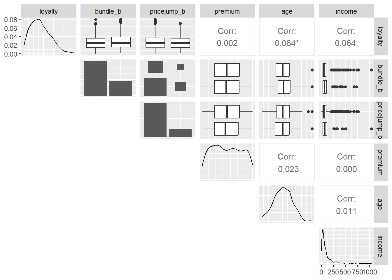
skim(sim_train)
Data summary
Name sim_train
Number of rows 900
Number of columns 8
_______________________
Column type frequency:
factor 4
numeric 4
________________________
Group variables None

Variable type: factor

skim_variable n_missing complete_rate ordered n_unique top_counts
bundle_b 0 1 FALSE 2 FAL: 632, TRU: 268
pricejump_b 0 1 FALSE 2 FAL: 720, TRU: 180
mobile_b 0 1 FALSE 2 TRU: 463, FAL: 437
churn 0 1 FALSE 2 FAL: 726, TRU: 174

Variable type: numeric

skim_variable n_missing complete_rate mean sd p0 p25 p50 p75 p100 hist
loyalty 0 1 8.49 4.83 0.2 4.8 7.9 11.5 24.9 ▆▇▅▂▁
premium 0 1 1137.60 486.65 300.0 720.0 1120.0 1552.5 2000.0 ▇▇▆▆▇
age 0 1 40.08 9.52 18.0 33.0 40.0 47.0 71.0 ▂▇▇▃▁
income 0 1 87.72 106.29 0.0 30.0 50.0 100.0 1040.0 ▇▁▁▁▁

The regression results

model_sim_v2 <- glm(formula = churn ~ .,
        family = binomial(link = "logit"), data = sim_train)
summary(model_sim_v2)

Call:
glm(formula = churn ~ ., family = binomial(link = "logit"), data = sim_train)

Coefficients:
                  Estimate Std. Error z value Pr(>|z|)    
(Intercept)     -0.2202193  0.4613275  -0.477  0.63311    
loyalty         -0.1179751  0.0214055  -5.511 3.56e-08 ***
bundle_bTRUE    -0.6553063  0.2151626  -3.046  0.00232 ** 
pricejump_bTRUE  0.4985342  0.2054056   2.427  0.01522 *  
premium          0.0005120  0.0001806   2.834  0.00459 ** 
age             -0.0196931  0.0092299  -2.134  0.03287 *  
income          -0.0008402  0.0009273  -0.906  0.36491    
mobile_bTRUE    -0.0086937  0.1764525  -0.049  0.96070    
---
Signif. codes:  0 '***' 0.001 '**' 0.01 '*' 0.05 '.' 0.1 ' ' 1

(Dispersion parameter for binomial family taken to be 1)

    Null deviance: 883.84  on 899  degrees of freedom
Residual deviance: 815.98  on 892  degrees of freedom
AIC: 831.98

Number of Fisher Scoring iterations: 5
predicted_probs_range <- predict(model_sim_v2, newdata = data_scenario_range, type = "response")
predicted_probs_means <- predict(model_sim_v2, newdata = data_feature_means, type = "response")
round(predicted_probs_range,5)
      1       2       3       4       5       6 
0.00534 0.01495 0.04387 0.18364 0.48978 0.67269 
round(predicted_probs_means,5)
      1 
0.18077 
coef_table <- coef(summary(model_sim_v2)) 
coef_tbl  <-  as_tibble(coef_table)
Coeff_labels <- c("(Intercept)", "Loyalty, yrs", "Bundle?(T)", "Price Jumped?(T)", "Premium, $000s", 
                 "Age, yrs", "Income, $000s","Mobile?(T)")
coef_tbl <- cbind(Coeff_labels, coef_tbl)

# Using gt() to render a table
coef_tbl_gt <- coef_tbl %>% gt() |> 
    opt_table_font(stack = "humanist") |>
    fmt_number(columns = everything(),
               decimals = 3)
coef_tbl_gt |> 
    data_color(
        columns = 'Pr(>|z|)', 
        palette = c("darkseagreen1", "darkseagreen3", "darkseagreen4"),
        domain = c(0,0.05),
        na_color = "lightgrey"
    )
Coeff_labels Estimate Std. Error z value Pr(>|z|)
(Intercept) −0.220 0.461 −0.477 0.633
Loyalty, yrs −0.118 0.021 −5.511 0.000
Bundle?(T) −0.655 0.215 −3.046 0.002
Price Jumped?(T) 0.499 0.205 2.427 0.015
Premium, $000s 0.001 0.000 2.834 0.005
Age, yrs −0.020 0.009 −2.134 0.033
Income, $000s −0.001 0.001 −0.906 0.365
Mobile?(T) −0.009 0.176 −0.049 0.961

Evaluate with confusion matrix

predict_test_probs <- predict(model_sim_v2, sim_test, type = "response")

predict_test_class <- as.factor(ifelse(predict_test_probs > 0.40, "TRUE", "FALSE"))
CrossTable(sim_test$churn, predict_test_class,
           prop.chisq = FALSE, prop.c = FALSE, prop.r = FALSE,
           dnn = c("Actual", "Predicted"))

 
   Cell Contents
|-------------------------|
|                       N |
|         N / Table Total |
|-------------------------|

 
Total Observations in Table:  100 

 
             | Predicted 
      Actual |     FALSE |      TRUE | Row Total | 
-------------|-----------|-----------|-----------|
       FALSE |        75 |         2 |        77 | 
             |     0.750 |     0.020 |           | 
-------------|-----------|-----------|-----------|
        TRUE |        21 |         2 |        23 | 
             |     0.210 |     0.020 |           | 
-------------|-----------|-----------|-----------|
Column Total |        96 |         4 |       100 | 
-------------|-----------|-----------|-----------|

 
predict_test_class <- as.factor(ifelse(predict_test_probs > 0.32, "TRUE", "FALSE"))
CrossTable(sim_test$churn, predict_test_class,
           prop.chisq = FALSE, prop.c = FALSE, prop.r = FALSE,
           dnn = c("Actual", "Predicted"))

 
   Cell Contents
|-------------------------|
|                       N |
|         N / Table Total |
|-------------------------|

 
Total Observations in Table:  100 

 
             | Predicted 
      Actual |     FALSE |      TRUE | Row Total | 
-------------|-----------|-----------|-----------|
       FALSE |        67 |        10 |        77 | 
             |     0.670 |     0.100 |           | 
-------------|-----------|-----------|-----------|
        TRUE |        18 |         5 |        23 | 
             |     0.180 |     0.050 |           | 
-------------|-----------|-----------|-----------|
Column Total |        85 |        15 |       100 | 
-------------|-----------|-----------|-----------|


Visualization

I think the most typical plot shows one predictor (ie., one feature) on the X axis while holding the other features constant. In this case, I will use Loyalty.

# test set but varying loyalty while others constant
test_vary_loyalty <- data.frame(
    churn = sim_test$churn,
    churnn = as.numeric(sim_test$churn)-1,
    loyalty = sim_test$loyalty,
    bundle_b = as.factor(FALSE), # the rest the same
    pricejump_b = as.factor(FALSE),
    premium = mean(sim_test$premium),
    age = mean(sim_test$age),
    income = mean(sim_test$income),
    mobile_b = as.factor(TRUE)
)
    
test_vary_loyalty$predicted_probs <- predict(model_sim_v2, newdata = test_vary_loyalty, type = "response")

p1 <- ggplot(test_vary_loyalty, aes(x = loyalty, y = predicted_probs)) +
    geom_line(color = "red", linewidth = 1) +
    geom_jitter(aes(x = loyalty, y = churnn), color = "black", size = 2, width = 0.02, height = 0.02) +
    labs(y = "Probability of Churn", x = "Loyalty, yrs") +
    theme_minimal()

Visualize sigmoid

But I also wanted to try plotting the sigmoid (aka, logistic) function which is given by p = 1/[1+exp(-z)] where z is the linear combination of all features. You’ll notice that I appended (binded) five artificial observations merely to extend the sigmoid.

sim_train2 <- sim_train
last_rows_n <- 5
last_row <- tail(sim_train2, n = last_rows_n)
last_row$loyalty = rep(0,last_rows_n)
last_row$bundle_b = rep(FALSE, last_rows_n)
last_row$pricejump_b = rep(TRUE, last_rows_n)
last_row$premium = c(3000,5000,9000,12000,14000)
last_row$age = rep(18, 5)
last_row$income = rep(40,5)
last_row$mobile_b = rep(FALSE, 5)
last_row$churn = rep(TRUE, 5)
sim_train2 <- rbind(sim_train2, last_row)
sim_train2f <- sim_train2

sim_train2$bundle_b <- as.numeric(sim_train2$bundle_b) - 1
sim_train2$pricejump_b <- as.numeric(sim_train2$pricejump_b) - 1
sim_train2$mobile_b <- as.numeric(sim_train2$mobile_b) - 1

# Linear combination (logit) for each observation
sim_train2$logit <- as.matrix(sim_train2[, setdiff(names(sim_train2), "churn")]) %*% coef(model_sim_v2)[-1] + coef(model_sim_v2)[1]

# Prediction
sim_train2$predicted_probs <- predict(model_sim_v2, newdata = sim_train2f, type = "response")
sim_train2$churn <- as.numeric(sim_train2$churn) - 1

p2 <- ggplot(sim_train2, aes(x = logit, y = predicted_probs)) +
    geom_jitter(alpha = 0.5, color = "purple", size = 2, width = 0.02, height = 0.02) +
    geom_jitter(aes(x = logit, y = churn), color = "black", size = 2, width = 0.02, height = 0.02) +
    # Next plots the sigmoid function
    geom_line(aes(y = 1 / (1 + exp(-logit))), color = "red", linewidth = 1) +
    labs(y = "Probability of Churn", x = "Logit (Linear Combination)") +
    coord_cartesian(xlim = c(-5,5)) +
    theme_minimal() 

p1 + p2

Visualize the marginal effects

p3 <- plot(ggpredict(model_sim_v2,c("loyalty", "pricejump_b")))
p4 <- plot(ggpredict(model_sim_v2,c("loyalty", "bundle_b")))
p3 <- p3 + coord_cartesian(ylim = c(0,.6))
p4 <- p4 + coord_cartesian(ylim = c(0,.6))
p3 + p4

what_is <- ggpredict(model_sim_v2,c("loyalty", "pricejump_b"))
what_is
# Predicted probabilities of churn

# pricejump_b = FALSE

loyalty | Predicted |       95% CI
----------------------------------
      0 |      0.38 | [0.29, 0.48]
      5 |      0.25 | [0.20, 0.31]
     10 |      0.16 | [0.12, 0.20]
     15 |      0.09 | [0.06, 0.14]
     20 |      0.05 | [0.03, 0.10]
     25 |      0.03 | [0.01, 0.07]

# pricejump_b = TRUE

loyalty | Predicted |       95% CI
----------------------------------
      0 |      0.50 | [0.38, 0.62]
      5 |      0.36 | [0.27, 0.45]
     10 |      0.23 | [0.17, 0.32]
     15 |      0.15 | [0.09, 0.22]
     20 |      0.09 | [0.05, 0.16]
     25 |      0.05 | [0.02, 0.11]

Adjusted for:
* bundle_b =   FALSE
*  premium = 1137.60
*      age =   40.08
*   income =   87.72
* mobile_b =   FALSE

Numerical examples to help explain coefficient interpretation

int_test <- data_feature_means
int_test$loyalty = 0
int_test
  loyalty bundle_b pricejump_b premium      age   income mobile_b
1       0    FALSE       FALSE  1137.6 40.07667 87.72222     TRUE
predict(model_sim_v2, newdata = int_test, type = "response")
        1 
0.3753352 
int_test$pricejump_b = as.factor(TRUE)
predict(model_sim_v2, newdata = int_test, type = "response")
        1 
0.4972846 
int_test$loyalty = 1
predict(model_sim_v2, newdata = int_test, type = "response")
        1 
0.4678353 
int_test$loyalty = 10
predict(model_sim_v2, newdata = int_test, type = "response")
        1 
0.2331494 
int_test$pricejump_b = as.factor(FALSE)