library(tidyverse)
library(corrplot); library(ggcorrplot) # may not use
library(factoextra)

# source is free trial of S&P https://www.tiingo.com/
# This is approximately the S&P1500; i.e, large-, mid- and small-cap stocks
stocks1500 <- read_csv("k-means-set_v1_2.csv")

stocks1500 <- stocks1500 |> rename(
    market_cap = 'Market Cap',
    div_yield = 'Dividend Yield',
    gross_margin = 'Gross Margin',
    revenue_growth = 'Revenue Growth (QoQ)',
    rho_sp500 = 'Correlation to S&P 500',
    volatility = '1 Year Volatility',
    pe_ratio = 'P/E Ratio',
    debt_equity = 'Debt/Equity (D/E) Ratio',
    ROE = 'Return on Equity (ROE)',
    ROA = 'Return on Assets (ROA/ROI)',
    TSR_1year = '1 Year Return',
    rho_treasury = 'Correlation to U.S. Treasuries',
    enterprise_value = 'Enterprise Val',
    pb_ratio = 'P/B Ratio'
)

# remove outliers, observed ex post
stocks1500 <- stocks1500 |> filter(Ticker != "AMZN")
stocks1500 <- stocks1500 |> filter(!Ticker %in% c("PDD", "MELI", "NDAQ", "RCL"))

# filtering by market cap: important reduction here!
df <- stocks1500 |> filter(market_cap > mean(stocks1500$market_cap))
numeric_cols <- df |> select_if(is.numeric)
options(scipen = 999)

# because we're going to standardize the features
original_means <- colMeans(numeric_cols)
original_sds <- numeric_cols  |>  map_dbl(sd)

std_cols <- numeric_cols |>
  mutate(across(everything(), ~(. - mean(.)) / sd(.)))

df_std <- df |>
    select(Ticker, Name, Sector, Industry) |>
bind_cols(std_cols)Contents
- Retrieve stocks and standardize features
- Select features
- Elbow method for optimal clusters
- K-means clusters
- Visualized
- Unscaled centroids
Retrive stocks and standardize features
Select features
selected_features <- c("volatility", "TSR_1year")Elbow method for optimal clusters
compute_elbow <- function(df, selected_columns) {
    numeric_data <- select(df, all_of(selected_columns))

    compute_wss <- function(k) {
        kmeans_result <- kmeans(numeric_data, centers = k, nstart = 25)
        kmeans_result$tot.withinss
    }

    k_values <- 1:25
    wss_values <- map_dbl(k_values, compute_wss)

    elbow_data <- tibble(k = k_values, wss = wss_values)

    # Calculate slopes
    elbow_data <- elbow_data %>%
        mutate(slope = c(NA, diff(wss) / diff(k)))

    return(elbow_data)
}

elbow_data <- compute_elbow(df_std, selected_features)

plot_elbow <- function(elbow_data) {
    ggplot(elbow_data, aes(x = k, y = wss)) +
        geom_line() +
        geom_point() +
        geom_text(aes(label = round(slope, 1)), vjust = -1.5) +
        theme_minimal() +
        labs(title = "Elbow Method for Optimal Number of Clusters",
             x = "Number of Clusters (k)",
             y = "Total Within-Cluster Sum of Squares")
}

# Use the function with your data
elbow_plot <- plot_elbow(elbow_data)

# Display the plot
print(elbow_plot)
K-means clusters
set.seed(9367) # Set a random seed for reproducibility

# Color palette
# location (ex post): top-middle, bottom-middle, bottom-right, left, top-right
custom_colors <- c("blue1", "darkorange1", "firebrick3", "cyan3", "springgreen3")

numeric_data <- df_std |> select(all_of(selected_features))

# based on the elbow method's so-called
# elbow point but ultimately is discretionary
num_clusters <- 5

kmeans_result_n <- kmeans(numeric_data, centers = num_clusters, nstart = 25)

# Print out the results
print(kmeans_result_n)
K-means clustering with 5 clusters of sizes 68, 69, 30, 85, 30
Cluster means:
volatility TSR_1year
1 -0.1663365 0.6846281
2 0.0751603 -0.6467280
3 1.7067078 -0.1904547
4 -0.9749478 -0.6417393
5 1.2598050 1.9443669
Clustering vector:
[1] 1 5 1 1 1 4 1 4 2 4 5 1 4 5 3 2 1 1 4 4 4 2 4 1 4 1 4 1 2 2 4 1 2 1 2 2 2
[38] 5 2 4 1 3 4 4 2 3 4 1 2 2 5 4 2 2 5 2 4 4 2 2 4 4 2 1 2 4 2 1 2 4 4 2 2 4
[75] 2 2 4 5 1 5 4 2 4 1 5 4 4 4 2 5 1 2 4 4 1 5 4 4 2 4 1 4 1 1 5 2 5 2 1 3 1
[112] 4 3 3 4 2 2 4 4 4 4 5 4 2 1 5 5 4 4 5 1 3 2 1 4 1 2 4 1 1 2 1 1 3 4 1 1 1
[149] 3 3 3 1 2 3 5 1 4 1 1 4 2 4 1 5 1 4 2 4 1 3 2 4 3 2 3 4 1 2 3 3 1 4 4 3 4
[186] 5 1 3 2 2 3 3 3 1 1 2 4 3 4 2 2 4 1 4 2 4 4 2 4 4 4 5 1 1 2 2 2 2 4 4 3 1
[223] 4 3 1 1 4 1 3 1 5 3 1 3 4 2 2 1 5 5 4 5 4 4 2 2 4 2 1 1 2 2 4 4 4 2 3 1 5
[260] 1 2 1 2 1 4 3 2 1 5 1 5 4 2 5 2 4 2 5 4 4 1 4
Within cluster sum of squares by cluster:
[1] 29.48504 27.95429 21.43397 27.33563 27.48363
(between_SS / total_SS = 76.2 %)
Available components:
[1] "cluster" "centers" "totss" "withinss" "tot.withinss"
[6] "betweenss" "size" "iter" "ifault" # attach cluster membership back to the original data
df_std$cluster <- kmeans_result_n$cluster
df$cluster <- kmeans_result_n$cluster
# Calculate mean and standard deviation for each feature, grouped by cluster
cluster_summary <- df |>
group_by(cluster) |>
summarise(across(everything(),
list(mean = ~mean(.), sd = ~sd(.)),
.names = "{.col}_{.fn}"))
# View the results: below instead
# cluster_summary$volatility_mean
# cluster_summary$volatility_sd
# cluster_summary$TSR_1year_mean
# cluster_summary$TSR_1year_sd
# cross_tab <- table(df_std$Sector, kmeans_result_n$cluster)
table(df_std$Sector, kmeans_result_n$cluster)
                          1  2  3  4  5
  Basic Materials         6  4  3  1  2
  Communication Services  3  3  0  3  0
  Consumer Cyclical       4  2  4  0  4
  Consumer Defensive      2  8  1 13  0
  Discretionary           0  1  0  0  0
  Energy                  9  4 13  4  2
  Financial Services     12 18  3 10  7
  Healthcare              3  4  0 17  1
  Industrials            14  8  0 17  4
  Real Estate             3  4  0  3  0
  Technology             10  7  6  3 10
  Unknown                 1  0  0  1  0
  Unknown Sector          1  3  0  1  0
  Utilities               0  3  0 12  0
Visualized
# Plotting
ggplot(df_std, aes(x = volatility, y = TSR_1year, color = as.factor(cluster))) +
    geom_point() +  # Add points
    stat_ellipse(type = "norm", level = 0.95) +
    geom_smooth(method = "lm", se = FALSE, color = "black", linetype = "dashed") +
    scale_color_manual(values = custom_colors) +  # Use custom color palette
    theme_minimal() +  # Minimal theme
    labs(color = "Cluster",
         title = "K-means clustering with only 2 features",
         subtitle = "Features are scaled",
         x = "Volatility",
         y = "1 year TRS (TSR_1year) ")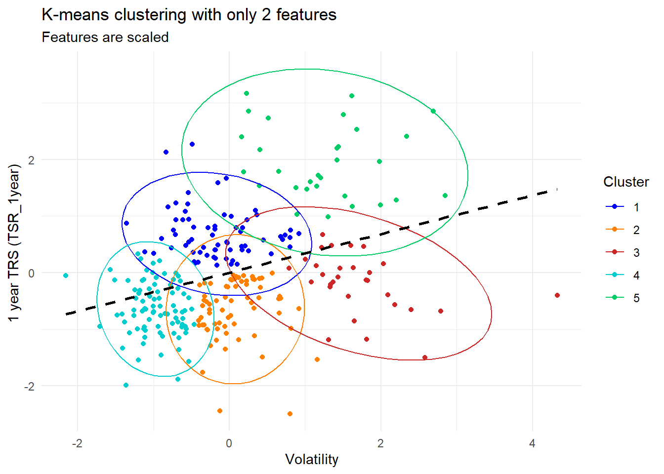
model_lm <- lm(TSR_1year ~ volatility, data = df_std)
corr <- cor(df_std$TSR_1year, df_std$volatility)
Unscaled centroids
selected_means <- original_means[selected_features]
selected_sds <- original_sds[selected_features]

scaled_centroids <- kmeans_result_n$centers

# Element-wise multiplication of each column by the corresponding standard deviation
# Then, addition of each column by the corresponding mean
unscaled_centroids <- sweep(scaled_centroids, 2, selected_sds, FUN = "*")
unscaled_centroids <- sweep(unscaled_centroids, 2, selected_means, FUN = "+")

unscaled_centroids_df <- as.data.frame(unscaled_centroids)
rownames(unscaled_centroids_df) <- paste("Cluster", 1:nrow(unscaled_centroids_df))

# sort by volatility
unscaled_centroids_df <- unscaled_centroids_df[order(unscaled_centroids_df$volatility), ]

print(unscaled_centroids_df)
volatility TSR_1year
Cluster 4 0.2438719 -0.04716554
Cluster 1 0.3173974 0.26064020
Cluster 2 0.3393562 -0.04832325
Cluster 5 0.4470738 0.55298364
Cluster 3 0.4877098 0.05756260